Using Deep Learning to classify Camera-Trap images from the African Jungle

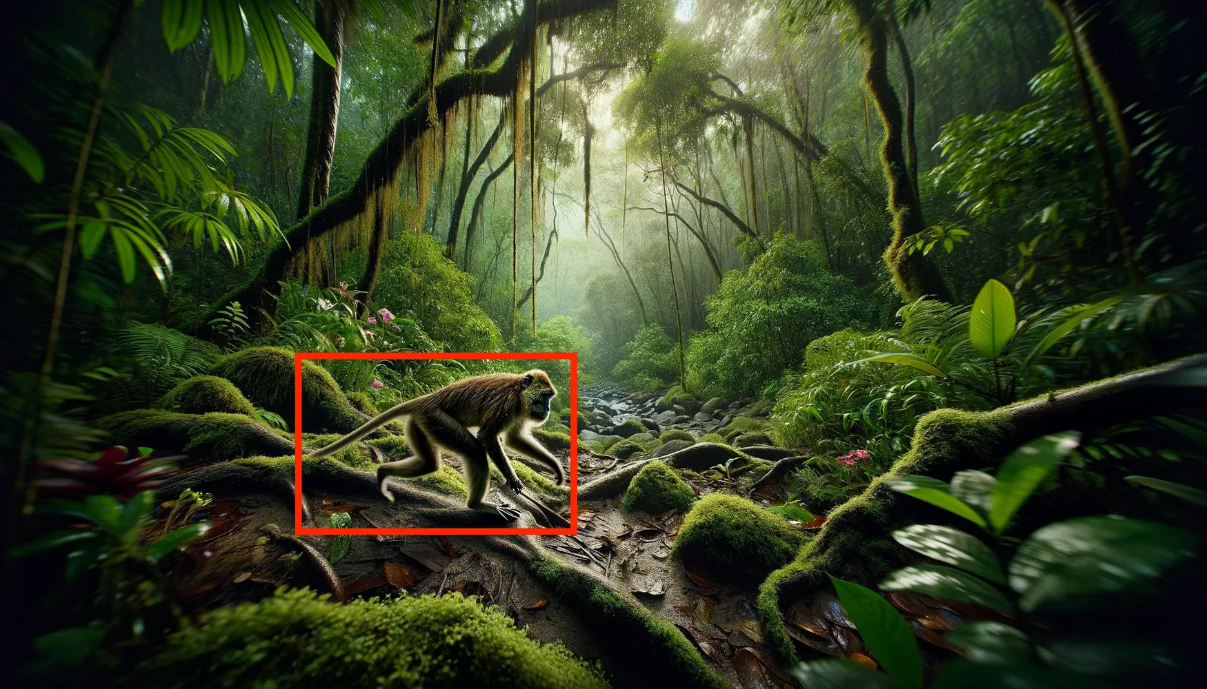
Embarking on an exploration through the African jungle isn’t an easy feat—even less so when embarked upon through the lenses of wildlife cameras. These cameras capture the untamed life of a world mostly unseen by human eyes, generating images rich with potential insights. The question is, how can we harness the power of Deep Learning to sort through this wilderness of pixels and accurately classify each creature that crosses the camera’s path? That’s exactly where the project took root.

My colleagues and I aimed to develop a computer vision-based solution capable of distinguishing among species captured in thousands of photos, automating what has historically been a manual task for wildlife researchers.

Throughout this blog post, we will dive into our journey, the solutions we discovered, and the wild ride that landed us a spot among the leaders in an international challenge dedicated to wildlife image classification.

The Purpose of the Project

Our project aimed at creating an intelligent solution to assist researchers in the rapid and accurate classification of wildlife species from camera trap images in Taï National Park. Our goal was to contribute to the conservation efforts by using Deep Learning to process the voluminous data generated by these traps, a task that usually relies heavily on the meticulous eyes of a human.

The challenge presented an array of seven distinct species that call the park home—birds, civets, duikers, hogs, leopards, other monkeys, and rodents—along with some empty frames devoid of any animals.

We were provided with a dataset rich with image data coupled with certain attributes intended to train and test our model. With images systematically categorized into training and testing sets, we had a solid foundation to start developing our models. Crucial here was the condition that our model needed to generalize well to previously unseen contexts since the training and testing sites were completely distinct.

The competition placed strict restrictions that no external dataset outside what was provided could be utilized, although leveraging publicly available, pre-trained computer vision models was allowed. Our goal was clear: develop a model that could stand the test of new contexts and help transform the way we protect and study the rich biodiversity of Taï National Park.

Challenges of Wildlife Image Classification

Classifying images from wildlife cameras stationed deep in the African jungle presents a unique set of challenges, this is illustrated by the diversity in our dataset.

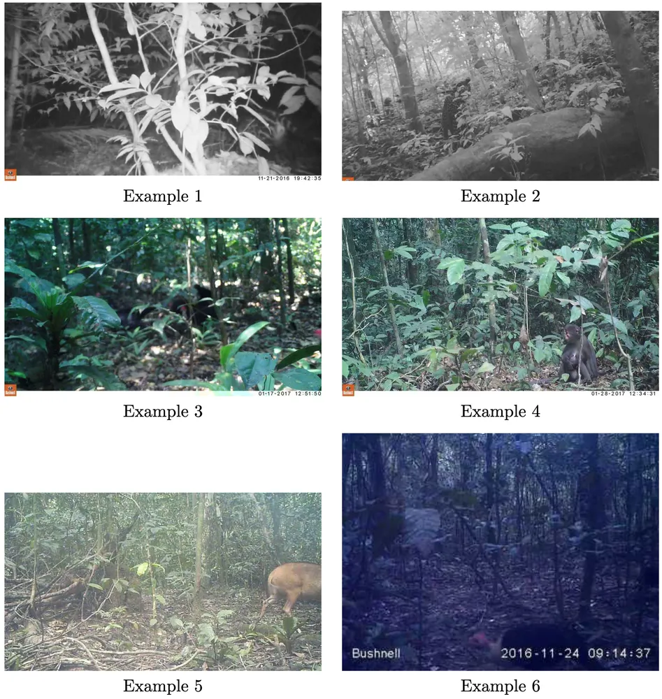
Firstly, let’s consider the lighting conditions. In the dataset, we encountered images similar to the ones above, where the first two are in black and white. The first example image is slightly overexposed, with the animal only partially visible. Whereas the second image is of good quality, but again only shows a small part of the animal. These varying exposures significantly increase the required complexity of classification models.

Next, we face issues with focus and clarity. Example image three is particularly difficult, due to the foreground foliage being the only part in sharp focus, with our subject of interest, the animal, appearing blurred in the background.

Moreover, the composition of the photographs is unpredictable. We have example image five, which captures the animal in motion, only halfway in the frame, meaning that our model would have to be robust against partial views of subjects. Meanwhile, the sixth image shows different lighting from the previous ones. This variation has to do with the time of the snapshot was taken. While the animal is distinguishable, the image quality is compromised.

Additionally, some images included metadata as text on the picture itself, a potential source of confusion for the models, which have to distinguish between relevant information and irrelevant on-screen clutter.

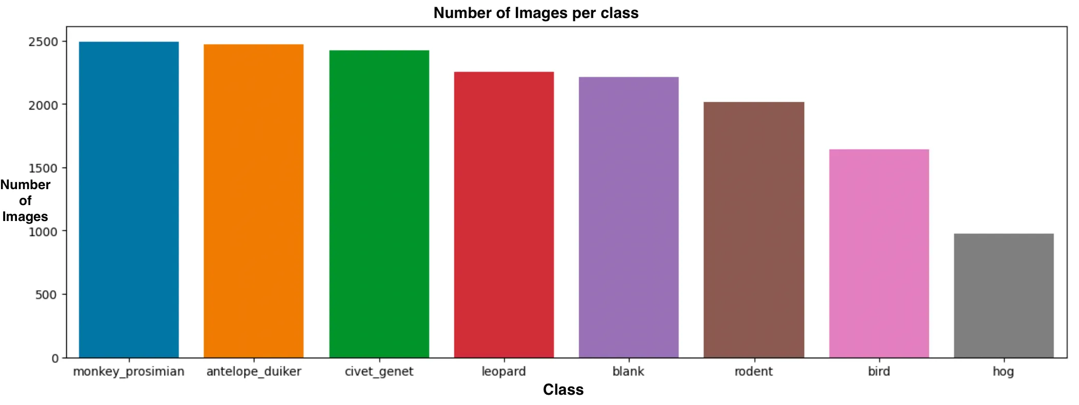
In addition to the difficult conditions of the image itself, the model was going to have to counter a significant class imbalance in the training data. The hog class, for example, had very few appearances in the dataset, which meant we were working against a natural bias that the model would generate during training.

Our deep learning models had to be adept at navigating through a multitude of complications including imperfect lighting, motion blur, partial animal sightings, diverse focus planes, and irrelevant textual data.

The International Challenge

Within the international arena of AI research, my team entered a competition aimed at pushing the boundaries of computer vision and deep learning as it applies to ecological monitoring. As part of a DrivenData Challenge leveraging a large array of camera trap images from various regions of Taï National Park, the challenge pushes the development in wildlife image classification.

My team and I worked over the course of several months, tweaking and evolving our approach in response to the leaderboard. This exercise wasn’t only a matter of academic interest, but a real-world application with the potential to impact conservation strategies and biodiversity research.

Over the last few months, we managed to retain the third spot in the worldwide challenge. This shows that we managed to develop an effective, robust solution that could be applied to real-world scenarios.

Applied Technologies

To accomplish our goal, we employed a set of powerful hardware and software tools to enable rapid experimentation and result analysis.

We chose Python 3.10 for its rich ecosystem of libraries and straightforward syntax, which is particularly well-suited for machine learning and data science related tasks.

To manage our experiments, we relied on Weights & Biases, an essential tool for tracking metrics, outcomes, and predictions. It provided us with a clear overview of our models’ performance in relation to their hyperparameters, thereby enabling us to pinpoint which adjustments led to improvements in performance.

When it came to machine learning frameworks, we integrated Pytorch Lightning into our workflow. Pytorch Lightning offers a class-based structure, bringing clarity to our deep learning projects. It simplifies the integration with Weights & Biases and significantly reduces boilerplate code, making our codebase cleaner and more maintainable.

Data Preprocessing

To mitigate the risk of overfitting our models to the training data, we implemented a transformation strategy as part of our regularization approach. Every iteration during training, these transformations would slightly alter the data and, consequently, the data’s gradient, enhancing the model’s ability to generalize to unseen images.

def _get_augmented_transform(image_size: int):
    return transforms.Compose(
        [
            transforms.Resize((image_size, image_size)),
            transforms.RandomHorizontalFlip(),
            transforms.ColorJitter(),
            transforms.ToTensor(),
            transforms.Normalize(mean, std),
        ]
    )

In the training phase, our function _get_augmented_transform applied a series of image processing operations, known as transformations, to each image. The sequence in which these transformations were listed in the function defined the order of their application, which included:

• Resizing: Adjusting the size of every image to a specified image_size to ensure consistent dimensions across all images. This is a crucial requirement for most computer vision models which need fixed input dimensions.

• Random Horizontal Flip: This transformation randomly flipped images horizontally, aiming to improve the model’s robustness to the varied horizontal orientation of animals in the images.

• Color Jitter: This transformation introduces random color variations to the image.

• Conversion to Tensor (ToTensor): This converted the image from its original format (which was a PIL Image) into a PyTorch Tensor, making it compatible with PyTorch models.

• Normalization: By subtracting the mean and dividing by the standard deviation, the images were normalized to improve numerical stability and ensure feature scales were consistent.

These transformation techniques were used to enrich training data diversity and quantity, increase the model’s robustness, and to avoid overfitting.

def _get_transform(image_size: int):
    return transforms.Compose(
        [
            transforms.Resize((image_size, image_size)),
            transforms.ToTensor(),
            transforms.Normalize(mean, std),
        ]
    )

For validation and test data, we defined a reduced version of these transformations. Since overfitting is not a concern with data that is not directly learned by the model, and our aim was to predict these images as accurately as possible, only Resize, ToTensor, and Normalize were used. This approach kept the validation and test data consistent with the training data concerning size and color space.

Deep Learning Models

We knew that the right model could mean the difference between a rough guess and an accurate prediction. Recognized for their ability to make sense of complex and high-dimensional data, deep learning models have excelled in computer vision tasks, making them ideal for our challenge.

In selecting a modeling approach, we relied on the power of transfer learning. This technique allowed us to take advantage of pre-trained models that had already learned visual representations from large datasets such as ImageNet. By fine-tuning these models on our specific dataset, we could reach higher accuracy levels more quickly than training from scratch.

On the one side, deeper and more complex models can understand a wide range of features and interactions, but could be more prone to overfitting without sufficient regularization. On the other hand, simpler models may miss out on subtle patterns in the data.

The Models We Experimented With

We experimented with a range of architectures, each with its own advantages and disadvantages:

ResNet-50, known for its residual learning framework which facilitates deeper network training by allowing feature reuse through skip connections, offered a promising foundation and robust performance on image recognition tasks.

EfficientNetv2 caught our attention with its scalability and balance between depth, width, and resolution, bolstered by novel training strategies that could handle our challenging dataset efficiently.

We also leveraged the DenseNet-161 architecture, distinguished by its dense connectivity pattern where each layer receives additional inputs from all preceding layers and passes on its own feature-maps to all subsequent layers, aiming to strengthen feature propagation and encourage feature reuse.

VGG-19, with its simplicity and depth which had shown considerable success in large-scale image recognition challenges, served as a baseline to measure the benefits of more complex architectures, despite its higher computational cost.

Inception V3’s appeal lay in its asymmetric design, which allowed it to learn at multiple scales and apply convolutions of different sizes concurrently.

Lastly, the Vision Transformer (ViT) distinguished itself from its convolutional counterparts. As an attention-based model initially developed for natural language processing, ViT utilizes a self-attention mechanism to weigh the importance of different parts of the input data, a relatively new approach that holds promise for the intricacies of wildlife image classification.

Our model experimentation aimed not only at finding the most effective architecture, but also to gain insights into the demands of the wildlife classification domain. Each model contributes unique insights that would lead us closer to accurate image classification in the wild.

Selecting the Best Performing Model

In order to select the best performing models, we incorporated both the Log Loss and an expanded set of F1 scores.

We primarily utilized the Log Loss, or logarithmic loss function, a staple evaluation metric in many neural network frameworks, for its ability to quantify the accuracy of a classifier by penalizing false classifications. Its formulation emphasizes not just whether predictions are wrong, but also the extent of their deviation from the truth.

$$loss = -\frac{1}{N} \sum_{i=1}^{N} \sum_{j=1}^{M} y_{ij} \log(p_{ij})$$

The Log Loss is particularly expressive when dealing with probabilistic predictions of multiple classes, and for our project, it served as a direct link to the evaluation criteria used in the challenge for which we developed our models. It works by taking the predicted probability of the true class and applying the logarithm, reverting the negative sign since logarithms of probabilities yield negative values. The sum of these is then averaged across all observations, giving us a sense of model performance on an intuitive scale, the lower the Log Loss, the better.

$$F1 = 2 \cdot \frac{precision \cdot recall}{precision + recall}$$

In addition to Log Loss, we incorporated the family of F1 scores. The F1 score captures the balance between precision and recall, serving as a more human understandable metric of a model’s performance, especially for stakeholders not intimately familiar with machine learning. For our multi-class problem, we looked at three common variants: Micro-F1, Macro-F1, and Weighted-F1.

$$F1_{micro} = \frac{2 \cdot TP}{2 \cdot TP + FP + FN}$$

Micro-F1 aggregates performance across all classes, presenting a global view on true positives, false positives, and false negatives to calculate precision, recall, and thus F1. This approach is useful when there’s a class imbalance, as it ensures that all classes contribute equally to the final score.

$$F1_{macro} = \frac{1}{M} \sum_{i=1}^{M} F1_i$$

Macro-F1 instead considers each class independently when calculating precision and recall, averaging out the individual F1 scores. It gives equal weight to each class, regardless of their variability in size within the dataset, making it possible for minority classes to have as much influence on the score as the majority ones.

$$F1_{weighted} = \frac{1}{N} \sum_{i=1}^{N} \frac{TP_i}{TP_i + FP_i + FN_i}$$

The Weighted-F1 score refines the Macro-F1 approach by adjusting the influence of each class in accordance with the number of observations it includes. This offers a more nuanced evaluation that favors larger classes and is of particular benefit where data distributions are unequal across classes.

By considering both Log Loss and the family of F1 scores, we were able to gain a comprehensive understanding of our models’ capabilities. This combined approach not only identified the best-performing model based on predictive confidence but also highlighted its balance of precision and recall across the varied classes. The models that performed the best, were those that minimized Log Loss while maintaining high F1 scores, reflecting both accuracy and reliability in their predictions.

Discouraging Initial Results

Initially, despite meticulous optimization across all our models, we hit a plateau with a validation loss plateauing at around 1.25 to 1.30. No matter the tweaks we made, we couldn’t significantly push past this barrier. This realization led us to acknowledge that minor tuning of hyperparameters was not going to be sufficient. We recognized the need for more drastic changes in our approach to our overall methodology.

Cropping using Megadetector

While trying to significantly improve our methodology, we turned to the use of an additional model to crop subjects within the pictures before classification. Among other options like Yolo, we chose Megadetector for its prior training on camera trap data, which we believed, would yield superior results.

We performed a one-off cropping of all our images using Megadetector, found in Microsoft’s CameraTraps GitHub repository. Cropping is time-consuming, and we wanted to avoid this computation in every training session, therefore we only went through the process once and stored the results. Our images were cropped at varying certainty thresholds of 5, 10, 20, 35, and 50.

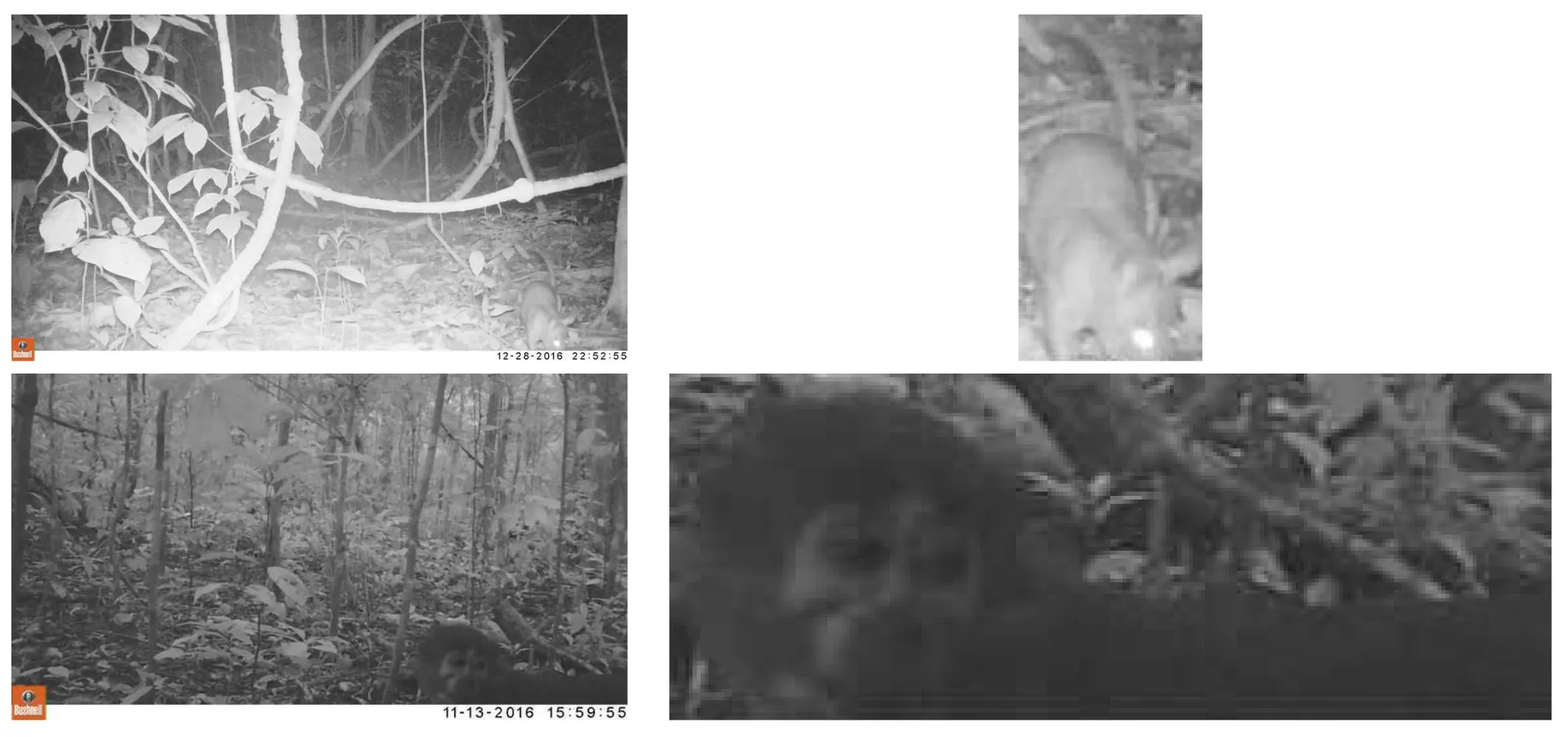
When we observe examples of cropped images, we were almost certain, that an improvement was imminent. Megadetector has proven itself as a great tool at focusing on the relevant subject in the frame, removing the bulk of unnecessary data. This fine-tuning has a significant upside, it allows our models to concentrate on pertinent details, which we anticipated would lead to a significant leap in our classification model’s performance.

Results and Analysis

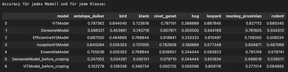
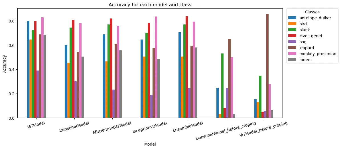
Following the cropping optimization using Megadetector, the Vision Transformer (ViT) emerged as the top-performing model. It achieved an F1-Weighted of 0.7569, an F1-Macro of 0.6678, and an F1-Micro of 0.7562, signaling consistent performance across classes. Its Log-Loss of 0.7816 also indicated a solid classification capacity.

Particularly impressive was the ViT model’s capability to classify antelope_duiker, civet_genet, and monkey_prosimian with accuracies surpassing 80%, showcasing excellent adaptability on our dataset. The lowest accuracy across models was observed for the hog class, suggesting this might be a challenging class to distinguish, possibly due to its limited representation in the dataset.

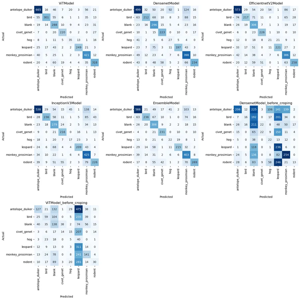
The confusion matrices for each model show correct predictions lined the main diagonal, while off-diagonal entries represented misclassifications.

We can see, that especially before cropping the images using Megadetector, most models had severe problems correctly classifying the images. The line becomes drastically more diagonal when we apply the cropping model before classifying.

Summary of Findings

After thorough analysis of the models, it is clear that cropping the images before classification significantly influenced model performance. The enhanced performance of post-cropping demonstrates the importance of preprocessing steps to eliminate irrelevant image information.

All models demonstrated commendable performance in identifying certain classes, though there is room for improvement in others, especially noticeable in the hog category, where all models showed low accuracy. A deeper examination of the data, specifically for this class, could potentially still enhance performance. Given that this class is the least represented in the dataset, a possible path of exploration would be to employ additional data augmentation techniques like copying existing data with slight modifications to increase the available amount of data.

Overall, we are highly satisfied with our models’ outcomes. All models performed adequately, notably in the classification of the monkey_prosimian category. The Vision Transformer (ViT) model, stands out in terms of accuracy, as well as F1 scores and Log-Loss. This demonstrates the effectiveness of the Transformer architecture in image classification, showcasing the potential power of Transformer-based models for image classification tasks.